Prototype Improved Reports from the Colorado Natural Resource Inventory
for the Bureau of Land Management
June 2002by Terence P. Yorks and Neil E. West
Department
of Rangeland Resources
Utah
State University
Logan, Utah 84322-5230
Purpose and Objectives
This report summarizes a project designed to summarize what alternative views of ecological condition, beyond those already produced, could be derived from a extensive set of BLM-NRCS data collected in western Colorado during the summer of 1997. All of the data pertaining to pinyon-juniper woodlands in that data set were examined and judgments made as to how scientifically defensible, and how costly, each data reduction process was. From this re-examination of a subset of about 70 of the 332 sampling units, we have been able to isolate additional error sources, produce several visually-effective data summaries, extrapolate how much time and money it would take to re-examine the entire data set, and determine the advisability of defending the particular techniques employed. This report includes examples from a variety of approaches, with appropriate commentary.
Notes on using this HTML-based report:
(1) Most graphed figures and tables have been converted from their original spreadsheet formats to ".pdf" hotlinks. Thereby, additional operating programs (other than the free-download Acrobat® Reader, which is typically already installed in browsers) or expertise are not required to view them. The conversion allowed the original designs to be preserved and to be quickly reached by a mouse-click on the underlined figure or table name, while being expandable in size in a way that directly included figures are not.
(2) If your screen is large enough to allow it, a particularly convenient way to view each hotlinked table and graph may be to right mouse click on its underlined link, and then select the "open in new window" option. In that way, the text and illustration may be set (or their windows moved) to be side by side, or however else is most convenient, and independently resized. Toggling among the windows may be done through the keyboard with the Alt-Tab combination, while added windows may be closed by Ctrl-W.
[Note, as of August 2007, that most browsers no longer do this easily; they now just download the pdf as a file.]
(3) Another way to pursue the report (and perhaps the easiest approach for the eyes) is to print just the text into hardcopy, and then use the computerized version to display the tables and figures. We have not solved the problem of how to make scientific text easily readable.
(4) Shifting back to a specific place in on-screen text from a figure or table should be possible either by using the Shift and left-arrow key combination, or via the browser "Back" icon, or through the browser menu (Go Back) function.
(5) Within tables or graphs, the zoom function (i.e., the "magnifier" icon in the browser/reader) may be necessary to resolve the contents clearly. Their initial visibility depends on the reader's screen- and window-size settings. Expanding the browser window size may help.
(6) Mention or use of trademarked or specific manufacture software or hardware does not imply an endorsement; specific identification is given for convenience in interpretation of what was done, and for potential replication or basis for improvement.
Background
The Natural Resource Conservation Service (NRCS) has been using resource inventories for over 60 years to assess the Nation's resources on private lands. The Rural Development Act of 1972 was the precursor to the institution of the modern USDA-NRCS National Resources Inventory (NRI). The Federal Land Policy and Management Act and the Public Rangeland Improvements Act mandate the USDI Bureau of Land Management (BLM) to complete a resource inventory of the public rangelands. Accordingly, within the BLM, there has been considerable effort to develop methods to accomplish a national inventory. However, none of the efforts have been universally accepted and/or economically feasible. In order to approach the remaining problems, several field rangeland pilot studies have been conducted by the federal agencies to test new methods for rangeland inventories and assessments. For example, in 1996, NRCS conducted a study in Colorado, Texas, and New Mexico which incorporated the Rangeland Health Model, an inventory of plant species composition, soil identification, and identification of other environmental data on site.
A cooperative agreement was established between BLM and NRCS to test the new NRI Methodology, which included the Rangeland Health Model, on 7.6 million acres of Public Land in western Colorado in 1997. The NRCS provided the initial statistical design for the project which was consistent with the National NRI assessment platform. Field data were collected by four interagency crews of three people each (one soil scientist and two vegetation specialists) at 332 sites throughout the western part of the state from June 1 until mid-October, 1997. The field data represents six Major Land Resource Areas The field data were keypunched at Iowa State University, and have undergone statistical analyses and detailed evaluation (especially by Kenneth Spaeth of the NRCS in Boise, Idaho). However, significant inconsistencies remain within the data set itself, so that neither a completely satisfactory report nor a data access pathway for additional analyses or management use have been completed.
Two preliminary reports have been made:
Spaeth, K.E., Pierson, F.B., Pellant, M., and Thompson, D. 2000. Natural Resource Inventory (NRI) on BLM lands in Colorado: an evaluation of the rangeland health model. Abstracts of the 53rd Annual Meeting of the Society for Range Management, Boise, ID, pp. 33-34.
Pellant, M., Spaeth, K., and Shaver, P. 2000. Final report on the use of a modifed National Resources Inventory protocol on BLM managed lands in Colorado. Abstracts of the 53rd Annual Meeting of the Society for Range Management, Boise, ID, p. 57.Our task was to reexamine a sub-sample involving the approximately 70 sites where pinyon-juniper woodlands occur as a pilot study to provide information on the feasibility of going forward with an expanded reporting effort based on the full data-set.
Goals (for this proof of concept)
i.) The first phase was to import information databases from the BLM and the NRCS, and compare with example physical files from the original data collection effort, establish the feasibility of more effectively evaluating several types of information, and derive its correlations with health indicators, for the Pinyon-Juniper (P-J) vegetation type.
ii.) The second phase was to suggest, once more familiarity with the P-J data set was gained, corrective factors for apparently consistent, and other specific, errors introduced into the data collection and transfer processes for the larger set of data.
iii.) From select corrected data, use statistical and graphical display computer packages to generate potential reporting formats that could be of increased utility to BLM managers, other agencies, and the public.
Data Error Findings - and Means to Resolve Them
One of the first steps in preparing for effective re-analysis was to create, using ArcView®, an interactive map of the sites, which would provide a baseline perspective for the project, and upon which information could be overlain in a visually effective fashion. Using this, within the computer file with 341 non-zero geographic coordinates provided, we found 4 entries that had their latitude and longitude reversed, and one had a latitude outside the Colorado border. This is a 1.5% data-entry-generated error rate, at an unsubtle level, within the keypunched database. Plotting data in an output format appropriate to them (in this case, a map) makes such problems jump out quickly. A lookup filter (to define an acceptable range for each parameter) during data entry could catch this level of problems immediately, even if the personnel were not sophisticated enough to recognize inappropriate results on a display.
The presence of obvious error in the first file examined suggested that more subtle data entry mistakes are nearly certain to be present throughout the entries. Indeed, comparison of the original data sheets with the electronic plant data tables revealed a set of inconsistencies that took a great many hours on the part of both USU and the BLM cooperators to unravel. In assembling the electronic subsets forwarded to us, it turned out that much of the data among sites was unintentionally switched. Five out of 6 test cases indicated seriously inaccurate transcriptions at the species production level. The right amounts of data were present, but not the right data in the right places relative to row and column headers. Random rechecking of final tables to be used for analysis against the original forms was the effective method for error detection here.
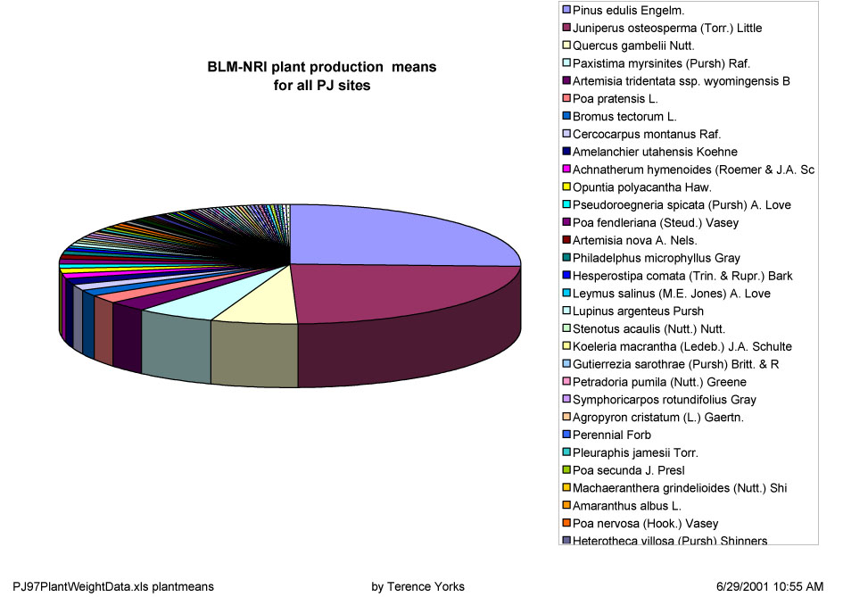
With that basic input data problem under apparent control, one of the next logical steps was to evaluate plant distributions among the PJ sites. A simple graph of overall mean production provided a couple of unexpected names as dominants. When plant production means were plotted (Figure 1, Growth),
[note added August 2007: since the browser problem has appeared, here is Figure 1 as a modest resolution example:]
and number of sites where particular species were found were visually examined in tabular format versus species rank, the 4th ranked species (Paxistima myrsinites (Pursh Raf.) was found to be present on just two sites, with almost all of it on only one site. The 10th ranked (Philadelphus microphyllus Gray) was similarly singularly represented on the same site. Neither species was anticipated to be common in PJ woodlands, from previous experience or the literature. Once again, plotting values against a function, given a basic understanding of what should be expected, leads to more certain error detection.Investigation of the original forms while chasing the above likely errors underlined what had already been known about the original study effort, that data collection groups had not consistently applied intended correction factors for plant production. It became clear as the electronic translations were compared to original data sheets that adjustments had been made to compensate, but not consistently, and without annotation of what changes were made when (i.e., metadata). Further changes by us or others would merely complicate the problem without knowledge of what has been done where and why. Going back to the original data sheets and starting over is hardly efficient use of time.
The key suggestion for future data collection and analysis efforts, therefore, is for metadata records to be kept at each step of the process, like those routinely used in GIS construction. Ideally, each file would have an associated note identifying who put that data in, when, and where it was derived from. Each time a data point was modified, that change should be noted, in a sequential format, e.g., by an "comment" annotation, or if the changes were widespread, but a formal amendment to the methods description. A lot of work, seemingly, but a maze of changes becomes impossible to follow if something at least similar is not done. Keeping all file iterations when changes to data are made, if possible with an annotated list of how they differ, would be a good intermediate step.
That process, however desirable, would not correct the Paxistima myrsinites and similar problems without a site-by-site examination of data reasonableness. It stood out as a data-scaling, correction-factor application possibility, but leads also to the question of species recognition accuracy, especially at more subtle levels, by modestly trained crews. This is an area that many professionals do not like to talk about, but indications of less than perfection even by the best observers abound. The most reliable method is the collection of plant vouchers (specimens),checking of these by a herbarium, and rapid feedback to those making erroneous identifications. If appropriate checking of plant species identifications cannot be done, it would probably be better to collect and analyze data as growth form categories. If there is one knowledgeable person checking the field crews, the national plant list could be used for definitively deciding where each observed plant fits among growth forms. That same source could assist in choosing which name is appropriate.
Further issues of sample size and overall accuracy, along with other error handling, are discussed subsequently in this report.
Potentially Useful Outputs from the Data Analysis Process
Code Translation Tables
One of the immediate practical needs for most subsequent data users is to be able to quickly appreciate what the codes used for convenience of computer personnel in tables really mean. To pick one at random, "CRPARCL" might be useful as a shortcut, if one is sufficiently familiar with it, but somehow its practical meaning does not leap out to most people, even for those with strong technical expertise in generally related fields. Hence conversion tables were built in Microsoft® (MS) Excel [Table 1: Codes]. This table set first paired abbreviated or acronym column and row headers, sorted alphabetically by code, with their location in the National Resource Inventory Colorado Test Pilot Workbook 1997, by data entry worksheet number, the page where that worksheet was bound, and the page number locating any more detailed description. Columns were added to relate the headers to a more general data category, where the data were located in files forwarded to us, and where it was transferred internally for analysis. Definitions were not completed, but could be filled in as desired. Additional file pages (reached via clicking on the tabs at the bottom of the original worksheet) provide these relationships sorted as they emerged from worksheet files, and by general data category for additional quick reference.
These relationships of codes to their more detailed descriptions also were then made accessible via a relational database intermediate (built in MS Access), to provide that additional information, as desired, with or without individual query, for results tables. Code translations could be done as hotlinks from these tables when web, or other computerized, access to the data needing translation was desired. Such hotlinks could be upgraded further by scanning in the full manual(s), with subsequent direct access to the relevant pages.
Similarly, plant names were referred to within the project by their formal Latin formats, their common name, and by codes. Hence a cross-reference table was prepared [Table 2, SpeciesList (231k)], with a shorter example subset [SpeciesListDemo (26k)] also available. Each of the species in all forwarded files is included, with columns for Latin name, code, common name, growth form, longevity, origin (native or introduced), the weight correction factor expected to be employed within the NRI study (per a file forward by Ned Habich), and any alternative names (synonyms). The proper codes, common name, growth form, longevity, and origin were derived by individually checking the provided scientific names with the U.S. government database at http://plants.usda.gov/.
This translation file was created initially to be able to group plant data for comparison with range (ecological) site descriptions in analyses. It could have considerable use outside this project, especially as a base for expansion, as needed. It must be noted, however, that in its present state, it suffers from erratic truncation in the species name column, which resulted from various file transfer protocols. Those truncations are not uncorrectable, but are not trivial, especially in making automated matches in database applications, or for full utility in final outputs.
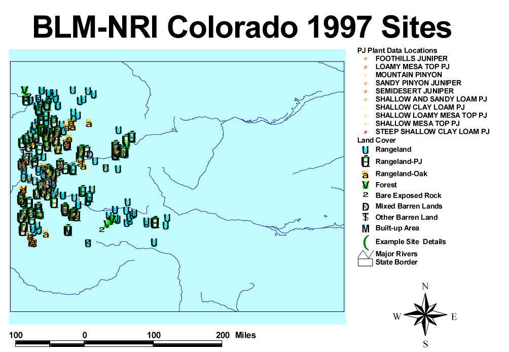
Overall Site Map
A table containing geographic location and land cover assignment was used as a baseline to create an ArcView® project file. Latitude and longitude were converted to decimal format in Excel, while state borders and major river locations were imported as a reference from files supplied with the ArcView program. An original goal was to interface the ArcView display set with DeLorme "3-D Topoquads" for the area, so that one could zoom into the various sites and visualize them in enhanced topographic richness, at almost any level of resolution desired. Alas, the best part of the DeLorme program did not work within our Windows NT operating system. Such an interface may be possible with Windows XP. An interface with the flat topographic map format could still be established.
Nevertheless, in the extant ArcView demonstration, the distribution of the sites and their basic cover attributes are made immediately apparent, and one can easily zoom in to differentiate sites that are hidden by symbol overlap at the initial full-state scale. [Note that the link required ArcView 3 or greater to run, and because of the file handling characteristics of that program, is not active in on-line versions of this report.] The pinyon-juniper data set is presented as a separate layer, as is an example single site. The latter has more complete, associated data that can be brought up by clicking on the table icon. Further, when the example site layer is active, clicking on the site location after the "hot link" icon is engaged will bring up a photograph of the site. This is a further demonstration of what could be accomplished throughout. Additional layers, and links to graphics or data, could be established readily, as desired for particular user groups.
ArcView is commonly available on government and other machines, but does have a significant learning curve and a variety of practical use problems, not least in file handling when moving a project from one machine to another, or to CD-ROM. Hence, an alternative example of output obtainable from ArcView is provided in .pdf format with this report (Figure 2, Overall Site Map).
[again added in August 2007 as a partial resolution image:]
Scanning Original Field Images - A Test Example
A set of 8 color prints, plus a key section of the topographic map, that were included in the original survey were scanned (using a UMAX Astra 1200S). All are included in the formal report folder ["Example Site"], with one reduced-size version presented here.
Basic scanning and correction during this process took somewhat less than 5 minutes per image, and thus about a half hour for the complete set. With our representative tool set, each image had to be hand-cropped, whether within the scanner preview step or by doing the cutting subsequently in Photoshop®. The former choice utilized less computer memory, but the latter made correcting color balance, orientation, and any other problems easier. Each image was scanned at 300 dpi (except for the map, @ 150 dpi), then had "auto-level" and "sharpen" applied in Photoshop, and was saved in .jpg format. Using .tif format resulted in four times larger files, and offered no visible improvement, but is requisite for active use with ArcView, and possibly for other purposes. For the map's file storage size, the color of the outline seemed to make little difference, nor did .gif vs .jpg format.
This overall scan and storage process resulted in 600 to 900 kb files for each image. A variety of rough tests indicated that anything visible to our unaided eyes on the original prints was also readable on the computer screen from the scanned and stored file at this resolution. Reducing these scanned images further to typical computer screen resolution of 72 dpi resulted in net file shrinkage to 55 to 90 kb.That size is still a bit large for web users who must work through a modem, but still left enough detail to be quite representative of the original image content for quick reference or general orientation purposes, as in the example above. Manipulation of the set in Photoshop on our Silicon Graphics computer did utilize >350 MB of active memory for a editing screen size of 1600x1200, more than many office machines have available at the moment.
Comparison of Plant Production Measurements to the Ecological or Range Site Descriptions
Table 3, MtnPinyon is set up as an example for data from a single ecological site. Its intent was to incorporate numerical plant production data with both conveniently truncated identifiers and fuller descriptions into a readily readable format on a computer screen (alternatively requiring very fine print to fit on 2 printed pages). In paralleling the traditional site descriptions, this table has been organized into growth form groups, with the assumption that within growth forms, the mean among sites would be the proper way to sort the individual species. To make comparisons more convenient, means for species are expressed in three columns: first as an absolute calculation from the NRI files, then as percent of overall site composition, and finally totaled to derive percentage composition by growth form.
The "Climax %" column in Table 3, MtnPinyon is derived from the 1989 draft range site description for Mountain Pinyon (#448). Only about half of the species anticipated from that draft document showed up in the NRI survey, but that comparison is complicated by possible differences in species naming, as well as accuracy in recognition. If this tabular approach were to be more routine, additions of the rest of the anticipated species and their percentages could become more useful. At the growth form level, the NRI indication is that graminoids are much lower and forbs somewhat lower, with shrubs and especially trees more prevalent, than the expectation for climax. The draft descriptions were written when the gradual, linear, deterministic and reversible Clementsian successional model to a single climax was commonly accepted. When these ecological site descriptions are modernized to include multiple stable states and transitions, the reference conditions may be expected to be quite different.
Additional columns, derived from another database, tie the Latin species name to the species code, common name, lifespan (longevity), and origin. These are followed by the individual sites' NRI by-species data, with totals calculated so that overall variance of production among sites can be viewed. A particularly useful part of this general form of presentation is that the unevenness of distribution of species among sites should be immediately apparent by visually scanning across this table. It may perhaps be even better seen this way than through the alternative approach of graphing. Scrolling about this table on a computer screen may be more effective than viewing it in print. The maintenance of detail by this approach, as opposed to statistical aggregation (e.g., means with high variances), allows useful information at the managerial level to be derived even when blind programs suggest that the results are too disparate for general conclusions to be made.
Graphs do have the advantage of condensation in physical output size, and through focus on single parameters. The most dominant species in overall production were displayed accordingly as proportional parts in Figure 3, MtPinyon Top10. Its display bars are ranked in order of total production among species. The unevenness of distribution should become especially apparent when viewing this graphical output in color. Each "series" (a word that the graphing software makes difficult to replace) simply represents one measurement site, and so color widths within each bar show the relative amount of production among sites. For example, nearly all the observed production of Poa spp. came from just one site, but was relatively high enough as to rank it 4th among all species when summed over all sites.
The reason for selecting just the top 10 may be seen in Figure 4, MtPinyon Inclusive, a graph which presents all the mean totals for species, divided proportionally by site within columns that have been ranked by total for all sites. This display does underline how much production is concentrated into a very few species.
However, going on to the next 12 species below the top 10 in Figure 5, MtPinyon Next reiterates how much variation there is among sites for individual species. This is not meant to indicate that there is any surprise in such a result, especially when site selection was randomized, but to show how the inherent variability can be made more easily apparent.
Visually scanning back to Table 3, MtnPinyon for the trees' portion first (and for the growth forms that are defined in the second column), and then for the other species within each form, should make comparisons even clearer and more provide more detail.
The utility of these approaches is that both a general idea and the particulars of output and plant diversity may be readily assessed and compared, by either practical users or scientists. It is paralleled by Figure 6, MtPinyon Means, a chart that gives the overall relative species distribution picture for Mountain Pinyon.
Similar species abundance displays were prepared for each of the ecological site types:
Foothills Juniper / Loamy Mesa Top / Mountain Pinyon / Sandy Pinyon Juniper / Semidesert Juniper / Shallow Clay Loam PJ / Shallow Loamy Mesa Top PJ / Shallow Mesa Top PJ / Shallow Sandy Loam PJ
An additional comparison (in a different presentation format) was done for the "Loamy Mesa Top PJ" ecological site type in Table 4, Plant Mass . Here, results for the sites surveyed are presented individually, displaying plant dry weights ranked according to their means across all surveyed sites. Mean percent composition was also calculated to make comparisons more straightforward with the values from the draft range site description, which have been typed at upper right. As with the other sites examined, the difference in species found versus species expected from the draft range site descriptions is striking.
Range vs. Tree Health
Another major question that we attempted to pursue was whether correlation existed between tree health and range health indicators. An MS Access database query was used to juxtapose the appropriate categories, with Excel for analyses and display, in Table 5, Range/Tree. This complex table divides data into rows according to tree health status within ecosystem types. The columns then reflect results for the outputs within each those separate tree health categories, searching for accuracy of correlations between tree health and range health indicators. Most standard deviations were in the 0.5 to 1 range for range health indicators. This means, assuming that + 2 standard deviations are required to indicate 95% inclusion within a normal distribution for full significance to be acquired, and with a total range of 0 to 5 for the range health category, not much statistical accuracy is likely from this data set (i.e., the variance is greater than the possible differences). This is not unexpected, given the high variance of results found in other areas of this study. Table 6, within this context of limited reliability, presents the results for range health indicators within tree health categories, along with the related number of trees within categories.
Properly weighting this type of comparison also becomes an almost impossible problem, since there are more tree health data plots than there are range health data plots. For statistical validity, one must work with groupings having no finer sums or averages than within the minimum size wherein the range health data were measured. However, even through this pathway, the weighting gets difficult, because the tree health breakdown may be uneven unless one is exceedingly careful in setting up the particular analysis path. Statistical programs are unlikely to automatically make the right kinds of choices. Example errors occurred in the database query from which this file was generated. Without special prompting, it calculated averages across the number of records that it encountered in the lowest level of each category within the report (e.g., disease within Foothills Juniper). That was not the proper result, which was an average across the total number of records within the ecological name. Still, it might be of interest to see how more lumping might change or simplify perception of differences in range health measures between sites with healthy trees and those categorized as other than healthy. Thus, additional tables were constructed for Table 7, Differences.
The high variance in the above approaches caused us not to pursue the range/tree health question further by a direct, traditional mathematical approach. This expression of analytic problems does not preclude gaining potentially useful information from the collected data. Figure 7, Tree Damage is an example of what may be derived without expectation of statistical significance, across all PJ sites. Tree height comparisons were also explored across sites via the relational database and an alternative presentation in Figure 8, Tree Sizes. Juniper results were distorted by an unusually high number of small, unhealthy trees at one location. The percentage of healthy or unhealthy trees could be displayed similarly. Specific locations of health problems, including those of a particular category, could also be directly connected to the ArcView map, and highlighted, to call attention to them if desired.
Similarly, for the range health indicators themselves, a series of graphs was constructed to display how they varied among ecosystem types, Figure 9 . For this figure, setting the Adobe Acrobat/Reader menu "View" option to "fit in window", or better, "full screen" (which the escape key will get one out of), one should be able to use page down and page up keys to flip through and compare among this series of graphs.
Sample Number
In reassessing the existing data after analysis, it became obvious that the number of samples which would be needed for statistical reliability would not have a single value. That key number, one of the particular targets that we were asked to investigate, will have a different variance for each characteristic being examined, as they are encountered in the field. Past management treatments are not, by any means, the only potential source of variance across seemingly comparable sites. The NRI-random-sample process was primarily designed for landscapes dominated by agriculture, within areas whose underlying characteristics (e.g., elevation, slope, aspect, soils, parent materials) tend to vary at a far less rapid rate over space than is encountered in untilled (wild) lands (especially those near or among mountains). Variations in these characteristics can easily overwhelm comparisons of management treatment (e.g., type of agriculture or grazing strategy) effects that are the goal of analyses. For example, consider the effects of south versus north facing slopes, that also may vary from 0 to 60 degrees, which are likely to be encountered frequently within an absolutely random site placement in wild lands, but rarely for agricultural fields. Just how important underlying conditions are for responses to treatment will vary with the parameter being investigated. In the end, required sample size will depend both on the question being asked and the subset being evaluated.
A rule of thumb for statistical analysis is that accuracy increases linearly with the square of sample size. Given the expense of data collection and data correction once collected, analytic statistical rigor for random sample location within complex topographic, treatment, and vegetation systems requires financial inputs that seem politically unlikely.
Looking to the future, the accusations of bias in sampling that the NRI process was created to address must be balanced against rationality of limits in underlying similarities and dissimilarities for sampling points. Absolute randomization is going to be a practical chimera for untilled lands with complex topography, at least until the costs of sampling are vastly less than at present. This does not mean that nothing can be learned from an investment in random sampling, even though standard statistical techniques are not likely to apply effectively in every context. Within this report are examples of a variety of tabular and graphic presentations of data that allow for useful interpretation of status and condition, and for comparisons across time and space, of managed rangelands that should be of interest to scientists, administrators, and the public.
Summary and Suggestions for the Future
As requested, we have explored the possibilities for deriving more conclusions from the 1997 BLM-NRCS test of expanding the NRI approach to assessing the ecological health of wild and other untilled lands in western Colorado. We looked at all of the data collected within pinyon-juniper woodlands there, hoping that some conclusions about that portion of the sample would emerge and help in addressing local needs. Unfortunately, we discovered too many inconsistencies and ambiguities in the basic data for us to have confidence in producing reliable new perspectives about these resources. We can, however, make some suggestions for designing more definitive assessments in the future.
Future assessments will be heavily scrutinized, particularly if changes in policies take place in response to the results of such assessments. If policy changes resulting from indications resulting from assessment are to withstand legal challenge [Science (2001) 293:189], then the assessment needs to be "transparent". By "transparent", we mean that a third party can verify that the assessment process can be run backward, from conclusions to primary data, and the same conclusions result from the re-analysis by the third party, as we have done here. If this process is impossible, then the results of the assessment will probably not withstand legal challenge. Thus, if such efforts are not to be voided, metadata, that is data about data, become extremely important. Because these metadata were missing in this test, we couldn't resolve some inconsistencies and ambiguities. We were, thus, frustrated in our efforts to re-analyze the data set at hand.
A defensible assessment has to be carefully designed through all the anticipated steps, from data collection, to data analysis and presentation of results. If counterintuitive results are reported, scrutiny will intensify. If a transparent process has not been employed, the results may not stand. It has been assumed in past that monitoring and assessment data could be aggregated upward, thus simultaneously answering questions as to extant conditions at numerous scales in time and space. Hierarchy theory (Lucid Update, http://www.fs.fed.us/institute/lucid, April 2001) is helping us realize that that is impossible in non-nested hierarchies. Non-nestedness is common in many aspects of wildlands. Thus, we may be forced to take separate approaches to monitoring national, regional, and local lands, depending on the variables we choose and their sensitivity to temporal and spatial scales.
If another NRI type approach is contemplated on BLM lands, we would suggest that one or a few key, well-experienced employees are put in charge well before any field work is undertaken. Furthermore, we suggest that these employees be assigned for the total duration of the project, including the data analysis and reporting phases. Rather than assign permanent agency personnel to do field sampling, we suggest that those tasks be bid out to contractors. This division of labor will encourage the BLM employees to have a more thoroughly thought out plan as the potential contractors will require more up front detail to make bids. The contractors will have to make all the logistical decisions as to how to get to the field sites, where to house and feed employees, whether to use trucks or helicopters etc. Thus, the BLM employees can focus on daily checks of the quality of data being turned in. Because these same BLM employees know they will be accountable for the final reports, there will be more attention paid to the details of the data being collected and its analysis. If the defendability of the final results are part of the performance record of these people and considered in their promotion, then the chances of unusable results lessen considerably.
In summary, although the furtherance of the understanding of the condition of federal wildlands and other untilled areas in western Colorado in 1997 was modest, we can learn from this attempt at re-analysis how such a campaign can be more successful in the future if different protocol are adapted. Thus, we suggest that little more attention be put on this past effort, although both hard copy and computer format data and preliminary results should be retained and kept accessible for interested researchers. Primarily, we should move on to more solid assessment designs in the future.
HTML text, design, and original figure transfers created on 28 June 2001,
most recently revised on 20 June 2002,
with example images added 16 August 2007,